本文共 6698 字,大约阅读时间需要 22 分钟。
http://www.xuebuyuan.com/2180573.html
1、排序和排名
根据条件对数据集排序(sorting)也是一种重要的内置运算。要对行或列索引进行排序(按字典顺序),可使用sort_index方法,它将返回一个已排序的新对象:
In [80]: obj = pd.Series(range(4), index=['d', 'a', 'b', 'c'])In [81]: obj.sort_index()Out[81]: a 1b 2c 3d 0dtype: int64
而对于DataFrame,则可以根据任意一个轴上的索引进行排序:
In [82]: frame = pd.DataFrame(np.arange(8).reshape((2, 4)), index=['three', 'one'], columns=['d', 'a', 'b', 'c'])In [83]: frame.sort_index()Out[83]: d a b cone 4 5 6 7three 0 1 2 3[2 rows x 4 columns]In [84]: frame.sort_index(axis=1)Out[84]: a b c dthree 1 2 3 0one 5 6 7 4[2 rows x 4 columns]
数据默认是按升序排序的,但也可以降序排序:
In [85]: frame.sort_index(axis=1, ascending=False)Out[85]: d c b athree 0 3 2 1one 4 7 6 5[2 rows x 4 columns]
若要按值对Series进行排序,可使用其order方法:
In [86]: obj = pd.Series([4, 7, -3, 2])In [87]: obj.order()Out[87]: 2 -33 20 41 7dtype: int64
在排序时,任何缺失值默认都会被放到Series的末尾:
In [88]: obj = pd.Series([4, np.nan, 7, np.nan, -3, 2])In [89]: obj.order()Out[89]: 4 -35 20 42 71 NaN3 NaNdtype: float64
在DataFrame上,你可能希望根据一个或多个列中的值进行排序。将一个或多个列的名字传递给by选项即可达到该目的:
In [90]: frame = pd.DataFrame({'b': [4, 7, -3, 2], 'a': [0, 1, 0, 1]})In [91]: frameOut[91]: a b0 0 41 1 72 0 -33 1 2[4 rows x 2 columns]In [92]: frame.sort_index(by='b')Out[92]: a b2 0 -33 1 20 0 41 1 7[4 rows x 2 columns] 要根据多个列进行排序,传入名称的列表即可:
In [93]: frame.sort_index(by=['a', 'b'])Out[93]: a b2 0 -30 0 43 1 21 1 7[4 rows x 2 columns]
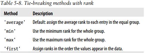
排名(ranking)跟排序关系密切,且它会增设一个排名值(从1开始,一直到数组中有效数据的数量)。它跟numpy.argsort产生的间接排序索引差不多,只不过它可以根据某种规则破坏平级关系。接下来介绍Series和DataFrame的rank方法。默认情况下,rank是通过“为各组分配一个平均排名”的方式破坏平级关系的:
In [95]: obj.rank()Out[95]: 0 6.51 1.02 6.53 4.54 3.05 2.06 4.5dtype: float64
也可以根据值在原数据中出现的顺序给出排名:
In [96]: obj.rank(method='first')Out[96]: 0 61 12 73 44 35 26 5dtype: float64
当然,你也可以按降序进行排名:
In [97]: obj.rank(ascending=False, method='max')Out[97]: 0 21 72 23 44 55 66 4dtype: float64
DataFrame可以在行或列上计算排名:
In [98]: frame = pd.DataFrame({'b': [4.3, 7, -3, 2], 'a': [0, 1, 0, 1], 'c': [-2, 5, 8, -2.5]})In [99]: frameOut[99]: a b c0 0 4.3 -2.01 1 7.0 5.02 0 -3.0 8.03 1 2.0 -2.5[4 rows x 3 columns]In [100]: frame.rank(axis=1)Out[100]: a b c0 2 3 11 1 3 22 2 1 33 2 3 1[4 rows x 3 columns]
2、带有重复值的轴索引
直到目前为止,我所介绍的所有范例都有着唯一的轴标签(索引值)。虽然许多pandas函数(如reindex)都要求标签唯一,但这并不是强制性的。我们来看看下面这个简单的带有重复索引值的Series:
In [101]: obj = pd.Series(range(5), index=['a', 'a', 'b', 'b', 'c'])In [102]: objOut[102]: a 0a 1b 2b 3c 4dtype: int64
索引的is_unique属性可以告诉你它的值是否是唯一的:
In [103]: obj.index.is_uniqueOut[103]: False
对于带有重复值的索引,数据选取的行为将会有些不同。如果某个索引对应多个值,则返回一个Series;而对应单个值的,则返回一个标量值。
In [104]: obj['a']Out[104]: a 0a 1dtype: int64In [105]: obj['c']Out[105]: 4
对DataFrame的行进行索引时也是如此:
In [107]: df = pd.DataFrame(np.random.randn(4, 3), index=['a', 'a', 'b', 'b'])In [108]: df Out[108]: 0 1 2a 0.863195 0.039140 0.328512a 1.387189 1.878447 1.899090b -1.239626 -0.256105 -0.699475b 0.325932 -0.834134 0.833157[4 rows x 3 columns]In [109]: df.ix['b']Out[109]: 0 1 2b -1.239626 -0.256105 -0.699475b 0.325932 -0.834134 0.833157[2 rows x 3 columns]
3、汇总和计算描述统计
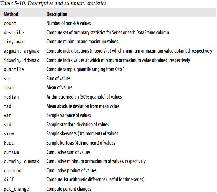
pandas对象拥有一组常用的数学和统计方法。它们大部分都属于约简和汇总统计,用于从Series中提取单个值(如sum或mean)或从DataFrame的行或列中提取一个Series。跟对应的NumPy数组方法相比,它们都是基于没有缺失数据的假设而构建的。接下来看一个简单的DataFrame:
In [110]: df = pd.DataFrame([[1.4, np.nan], [7.1, -4.5], [np.nan, np.nan], [0.75, -1.3]], index=['a', 'b', 'c', 'd'], columns=['one', 'two'])In [111]: dfOut[111]: one twoa 1.40 NaNb 7.10 -4.5c NaN NaNd 0.75 -1.3[4 rows x 2 columns]
调用DataFrame的sum方法将会返回一个含有列小计的Series:
In [112]: df.sum()Out[112]: one 9.25two -5.80dtype: float64
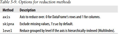
传入axis=1将会按行进行求和运算:
In [113]: df.sum(axis=1)Out[113]: a 1.40b 2.60c NaNd -0.55dtype: float64
NA值会自动被排除,除非整个切片(这里值的是行或列)都是NA。通过skipna选项可以禁用该功能:
In [114]: df.mean(axis=1, skipna=False)Out[114]: a NaNb 1.300c NaNd -0.275dtype: float64
有些方法(如idxmin和idxmax)返回的是间接统计(比如达到最小值或最大值的索引):
In [115]: df.idxmax()Out[115]: one btwo ddtype: object
另一些方法则是累计型的:
In [116]: df.cumsum()Out[116]: one twoa 1.40 NaNb 8.50 -4.5c NaN NaNd 9.25 -5.8[4 rows x 2 columns]
还有一种方法,它既不是约简型也不是累计型。describe就是一个例子,它用于一次性产生多个汇总统计:
In [117]: df.describe()Out[117]: one twocount 3.000000 2.000000mean 3.083333 -2.900000std 3.493685 2.262742min 0.750000 -4.50000025% 1.075000 -3.70000050% 1.400000 -2.90000075% 4.250000 -2.100000max 7.100000 -1.300000[8 rows x 2 columns]
对于非数值型数据,describe会产生另外一种汇总统计:
In [118]: obj = pd.Series(['a', 'a', 'b', 'c'] * 4)In [119]: obj.describe()Out[119]: count 16unique 3top afreq 8dtype: object
4、相关系数与协方差
有些汇总统计(如相关系数和协方差)是通过参数对计算出来的。我们来看几个DataFrame,它们的数据来自Yahoo! Finance的股票价格和成交量:
import pandas.io.data as weball_data = {}for ticker in ['AAPL', 'IBM', 'MSFT', 'GOOG']: all_data[ticker] = web.get_data_yahoo(ticker, '1/1/2000', '1/1/2010')price = DataFrame({tic: data['Adj Close'] for tic, data in all_data.iteritems()})volume = DataFrame({tic: data['Volume'] for tic, data in all_data.iteritems()}) 说明:
雅虎链接已经失效,不能访问获取数据。
接下来计算价格的百分数变化:
In [1]: returns = price.pct_change()In [2]: returns.tail()Out[2]: AAPL GOOG IBM MSFTDate 2009-12-24 0.034339 0.011117 0.004420 0.0027472009-12-28 0.012294 0.007098 0.013282 0.0054792009-12-29 -0.011861 -0.005571 -0.003474 0.0068122009-12-30 0.012147 0.005376 0.005468 -0.0135322009-12-31 -0.004300 -0.004416 -0.012609 -0.015432
Series的corr方法用于计算两个Series中重叠的、非NA的、按索引对齐的值的相关系数。与此类似,cov用于计算协方差:
In [3]: returns.MSFT.corr(returns.IBM)Out[3]: 0.49609291822168838In [4]: returns.MSFT.cov(returns.IBM)Out[4]: 0.00021600332437329015
DataFrame的corr和cov方法将以DataFrame的形式返回完整的相关系数或协方差矩阵:
In [5]: returns.corr()Out[5]: AAPL GOOG IBM MSFTAAPL 1.000000 0.470660 0.410648 0.424550GOOG 0.470660 1.000000 0.390692 0.443334IBM 0.410648 0.390692 1.000000 0.496093MSFT 0.424550 0.443334 0.496093 1.000000In [6]: returns.cov()Out[6]: AAPL GOOG IBM MSFTAAPL 0.001028 0.000303 0.000252 0.000309GOOG 0.000303 0.000580 0.000142 0.000205IBM 0.000252 0.000142 0.000367 0.000216MSFT 0.000309 0.000205 0.000216 0.000516
利用DataFrame的corrwith方法,你可以计算其列或行跟另一个Series或DataFrame之间的相关系数。传入一个Series将会返回一个相关系数值Series(针对各列进行计算):
In [7]: returns.corrwith(returns.IBM)Out[7]: AAPL 0.410648GOOG 0.390692IBM 1.000000MSFT 0.496093
传入一个DataFrame则会计算按列名配对的相关系数。这里,我计算百分比变化与成交量的相关系数:
In [8]: returns.corrwith(volume)Out[8]: AAPL -0.057461GOOG 0.062644IBM -0.007900MSFT -0.014175
传入axis=1即可按行进行计算。无论如何,在计算相关系数之前,所有的数据项都会按标签对齐。